How to Create a Universe: A Simple Starting Point of Running a Cosmological Simulation on your PC
This project originated from one of my master’s courses. The author is a student passionate about astrophysics but did not learn it systematically - any advice or constructive criticism is welcome!.
Example scripts will be uploaded to Github.
Have you ever imagined that someday create a universe of your own in your childhood? Have you ever heared that some scientists on our little blue planet are working on simulating how the universe forms and evolves? And have you realized that you could try to run your own simulation on your PC? This post is actually a guide of making a very very simple cosmological simulation code.
Step 1: Physical Scenario
Modern cosmology theory tells us:
The early universe had near-uniform matter distribution with tiny density fluctuations. Over hundreds of millions of years, gravity amplified these fluctuations - dense regions attracted more matter while voids lost material. Dark matter formed cosmic webs of filaments and halos, within which gas collapsed to form stars and galaxies, ultimately creating today’s universe of galaxy clusters connected by filaments, separated by vast voids. This gravitational dance continues shaping cosmic structure. This is the big picture of our simple simulation.
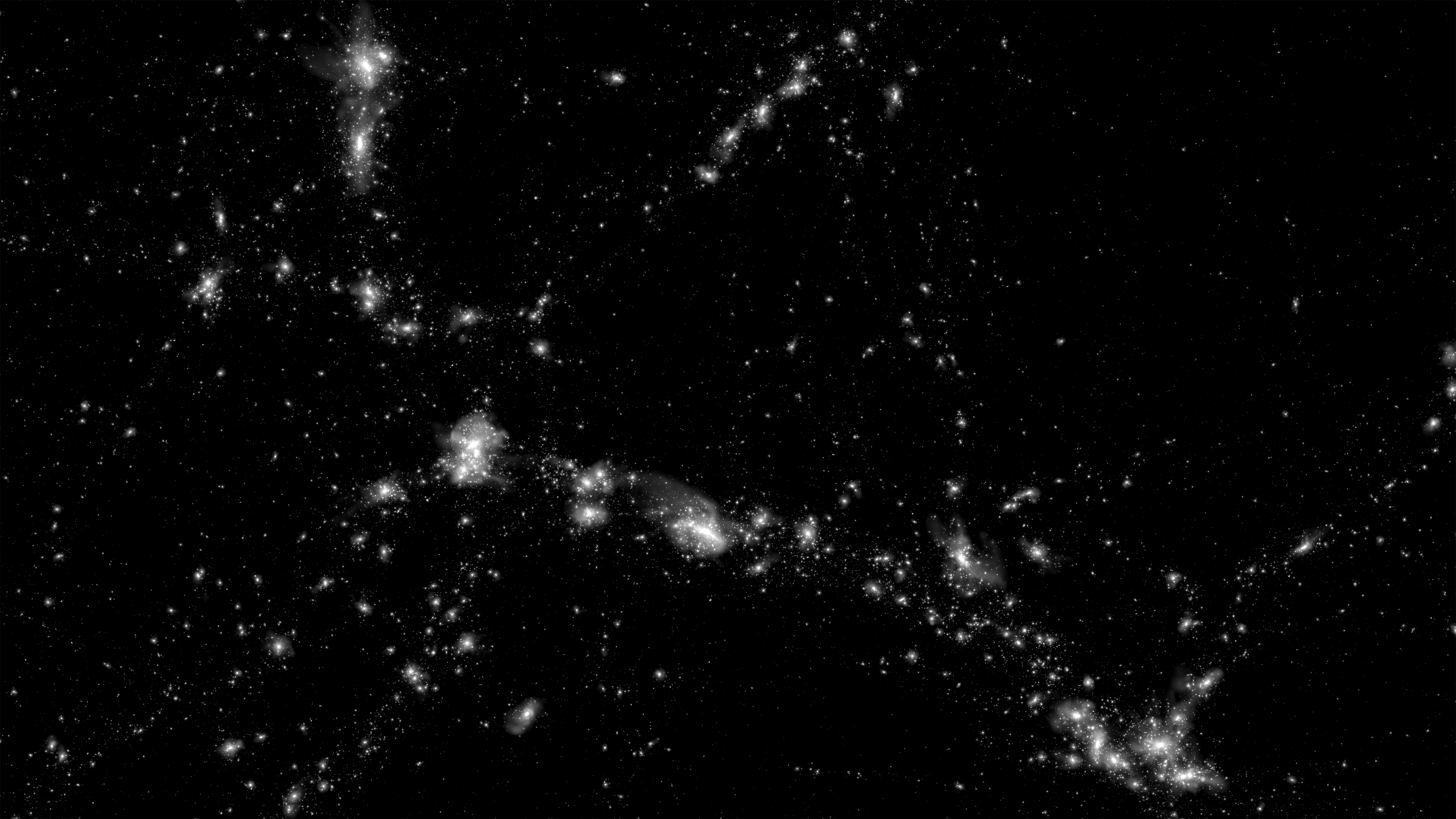
*This is how the large-scale stucture looks like. The figure is from IllustrisTNG project.
However, as a very very simple one, our simulation won’t consider all of these elements. We have some assumptions to simplify the situation.
Assumption 1: no cosmic expansion here. In order to reduce the computational cost, we do not consider the cosmic expansion. By the way, it could be experesssed as that our result just represents some certain region of our universe.
Assumption 2: only dark matter. This is one of the core assumptions of this simulation. On the one hand, dark matter is usually considered as some kind of mysterious collisionless, purely-gravitational particles, which means that we could save many computational resources: no collision, no Navier-Stokes equation, no chemical evolution… On the other hand, baryonic matters are not that important for a simplified simulation: although they dominate the feedback processes, they just take a very small fraction of our universe.
Assumption 3: this is a 2D universe. This is one of the core assumptions of this simulation as well. Reducing spatial dimensions:
· Cuts a lot of data storage needs.
· Maintains qualitative structure formation patterns
· Enables personal computer execution
Assumption 4: we adopt newtonian gravitation completely. It is very understandable as well: save resource and is still precise enough due to almost no relativistic process here(we even abandoned Friedmann equations!).
Step 2: Simulate your own universe
We have reviewed the basic physics of our simulation. Let’s translate physics into Python code (using Jupyter Notebook):
Block 1: some initial setup works
1
2
3
4
5
6
7
8
9
10
11
12
13
14
15
16
17
18
19
20
21
22
23
24
25
26
27
28
29
30
31
32
33
34
35
36
37
38
39
40
41
42
43
44
45
46
47
48
49
50
51
52
53
54
55
56
57
## Initial conditions
# ======================

import numba
import numpy as np
import matplotlib.pyplot as plt

# Setup the number of CPU cores of computation
numba.set_num_threads(16)

# Parameters
n = 120            # number of particles is n*n
L = 100.0         # Length of this universe
sigma = 1e-2 * L  # factor of primordial perturbations
r_cut = 20.0       # cut radius
softening = 0.4    # avoiding infinite gravitation
dt = 0.01          # time step
steps = 1000        # total steps
grid_size = 500  # girds of figures autosaved
v_factor = 1e0  # factor for Gaussian velocity field

# Create center coordinates of each grid
grid = np.linspace(0, L, n, endpoint=False) + 0.5 * L/n
x_centers, y_centers = np.meshgrid(grid, grid)

# Create Guassian random displacement field
np.random.seed(42)
dx = np.random.normal(0, sigma/np.sqrt(2), (n, n))
dy = np.random.normal(0, sigma/np.sqrt(2), (n, n))

# Periodic packing function
def periodic_wrap(pos, L):
    return pos % L

# Initial velocity and displacement fields
x_init = periodic_wrap(x_centers + dx, L)
y_init = periodic_wrap(y_centers + dy, L)

vx = v_factor * dx / sigma
vy = v_factor * dy / sigma

particles = np.stack([x_init.ravel(), y_init.ravel(), vx.ravel(), vy.ravel()], axis=1)

# Visulization
plt.figure(figsize=(20,10))
plt.subplot(121)
plt.scatter(particles[:,0], particles[:,1], s=0.05, c='b')
plt.title("Initial Positions")
plt.xlabel("x "), plt.ylabel("y ")

plt.subplot(122)
plt.quiver(particles[:,0], particles[:,1], particles[:,2], particles[:,3], scale=50)
plt.title("Initial Velocity Field")
plt.tight_layout()
plt.show()
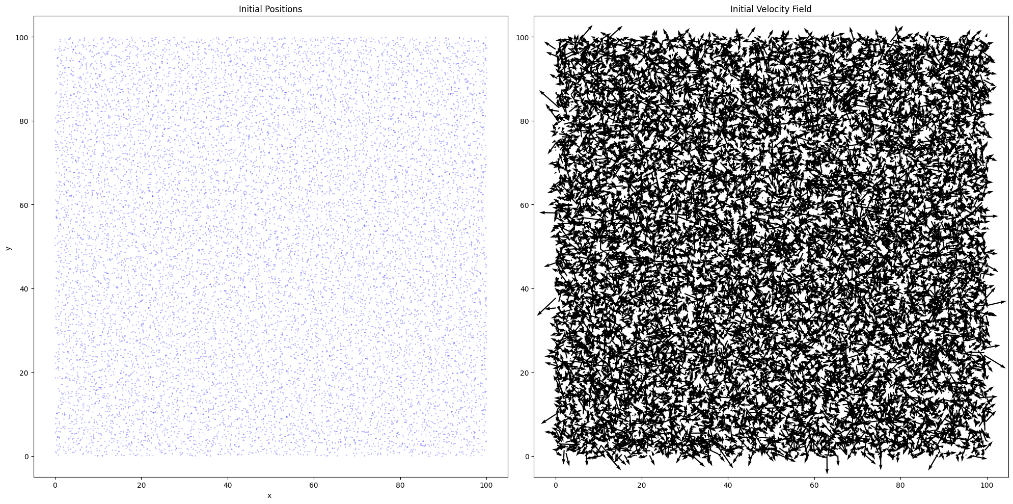
We create a 2D “universe box” with particles arranged in a near-uniform grid plus Gaussian perturbations, mimicking primordial density fluctuations from cosmic inflation. Key implementation notes:
· Gaussian displacements (dx, dy) model quantum fluctuations
· Perturbation amplitude (sigma): Controls structure formation speed
· Scale normalization: /np.sqrt(2) ensures proper variance distribution in 2D
· Initial velocity assumptions: Links initial velocities to density gradients
· Reproducibility: np.random.seed(42) enables parameter comparison
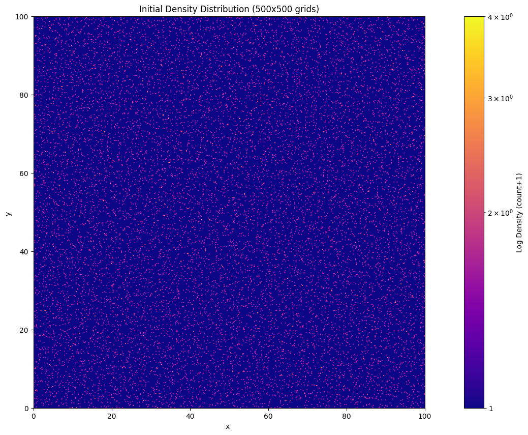
OK, let’s see the output:
Block 2: computing the gravitation
The code for computing the gravitation (more accurately, acceleration) among all the particles is as follows:
1
2
3
4
5
6
7
8
9
10
11
12
13
14
15
16
17
18
19
20
21
22
23
24
25
26
27
28
29
30
31
## Computing gravitation
# ======================

from numba import njit, prange

@njit(parallel=True, fastmath=True)
def compute_accelerations(positions, L, r_cut, softening):
    N = positions.shape[0]
    acc = np.zeros_like(positions)
    factor = (L**2) / N  # Equivalent to G*m

    for i in prange(N):
        pos_i = positions[i]
        for j in range(N):
            if i == j: continue  # Avoid to compute gravitation between a particle and itself

            # Periodic mirror
            delta = positions[j, :2] - pos_i[:2]
            delta -= np.round(delta / L) * L

            # Computing the distance
            r_sq = delta[0]**2 + delta[1]**2 + softening**2
            if r_sq < r_cut**2 and r_sq > 0:
                inv_r3 = 1.0 / (r_sq ** 1.5)
                acc[i, :2] += delta * inv_r3  # a ∝ 1/r²

        acc[i] *= factor  # Normalization

    return acc
Let me explain some important points: 1. njit is a method to increase computational efficiency. The effect depends on:
1
2
# Setup the number of CPU cores of computation
numba.set_num_threads(16)
The number(here 16) is the number of CPU cores you would like to use. So be aware of it, making sure to set a correct number.
2. We use softening length to avoid infinite gravitation. So you can change the value of it to test the effect. It would be interesting. Usually, a relatively small value will be better.
3. You might be confused about the introduction of factor. This is because we should let the average density be approximately irrelevant to the spatial scale L. We could see the areal density \(\sigma\) satisfies:
\[\sigma = \frac{N \cdot m}{L^2},\]where m is the mass of each particle; N is the total number of particles.
And according to the formula of acceleration, we could know factor here replaces G*m, let:
\[\frac{L^2}{N} = G \cdot m\]Then it is easy to see letting fatcor be current form could ensure the density irrelevant to L. You might ask why \(\sigma\) seems like equal to G. The reason is clear: all of these variables have been parameterized. The exact values are not important. The laws of their changes matter much more.
Block 3: update velocity, position and acceleration
The code:
1
2
3
4
5
6
7
8
9
10
11
12
13
# Update v, a, x
# ======================

# Leapfrog method
def leapfrog_step(pos, vel, acc, dt):
    vel_half = vel + 0.5 * acc * dt     # half new velocity
    pos_new = pos + vel_half * dt       # full new position
    pos_new = periodic_wrap(pos_new, L) # periodic boundary
    acc_new = compute_accelerations(pos_new, L, r_cut, softening) # full new acceleration
    vel_new = vel_half + 0.5 * acc_new * dt # full new velocity
    return pos_new, vel_new, acc_new
Leapfrog method advantages:
· Energy conservation (vs Euler method’s error accumulation)
· Phase-space accuracy
· Symplectic time-reversibility
Block 4: perform the calculations and save the results
1
2
3
4
5
6
7
8
9
10
11
12
13
14
15
16
17
18
19
20
21
22
23
24
25
26
27
28
29
30
31
32
33
34
35
36
37
38
39
40
41
42
43
44
45
46
47
48
49
50
51
52
53
54
55
56
57
58
59
60
61
62
63
# Perform the calculations and save the results
# ======================

def generate_heatmap(positions, L, grid_size):  # Grid size is here.

    bins = np.linspace(0, L, grid_size+1)
    density, _, _ = np.histogram2d(
        positions[:,0], positions[:,1],
        bins=(bins, bins)
    )

    # Normalize to [0,1]
    density = (density - density.min()) / (density.max() - density.min() + 1e-8)
    return density.T


# Simulation

import matplotlib.pyplot as plt
import os

output_dir = "./density_heatmaps"
os.makedirs(output_dir, exist_ok=True)

positions = particles[:, :2].copy()
velocities = particles[:, 2:].copy()

acc = compute_accelerations(positions, L, r_cut, softening)

# Perform the simulation
for step in range(steps):
    # Update
    positions, velocities, acc = leapfrog_step(positions, velocities, acc, dt)

    # Create heatmaps
    density = generate_heatmap(positions, L, grid_size)  # Grid size is here.

    # Avoid zero
    density += 1

    # Visualization
    plt.figure(figsize=(8,6))
    plt.imshow(density, origin='lower', extent=[0, L, 0, L],
              cmap='jet')#, norm=LogNorm(vmax=1.8))

    cbar = plt.colorbar(label='Log Density (count+1)')
    cbar.formatter = plt.LogFormatter()
    cbar.update_ticks()

    plt.title(f"Step {step+1}/{steps}, t = {(step+1)*dt:.1f}")
    plt.xlabel("x"), plt.ylabel("y")

    # Save
    plt.savefig(f"{output_dir}/heatmap_{step:03d}.png", dpi=150, bbox_inches='tight')
    plt.close()

    # Display the completion progress
    if (step+1) % 10 == 0:
        print(f"Saved heatmap {step+1}/{steps}")

print(f"All figures are saved in: {os.path.abspath(output_dir)}")
OKay. When you run the simulation, all figures will be saved in the folder you specified. Now we have completed the whole simulation. Although it is very simple and crude, it could roughly show the growth of structures(such as large-scale structures or several halos/ galaxies, depending on your parameters) under pure gravitation. It is funny, but have severe limitations. For example, we just simply ignored the cosmic expansion, and also, there is no feedback process due to the absence of baryonic components and black holes. Maybe you could try to add them on your computer ^_^
Last but not least, we can see one example gif of the result. It shows the growth and merger of several galaxies. Due to the limitation of this site, I just used a part of frames to create the gif. And the code is attached below as well:
1
2
3
4
5
6
7
8
9
10
11
12
13
14
15
16
17
18
19
20
21
22
23
24
25
26
27
28
29
30
31
32
33
34
35
36
37
38
39
40
41
42
43
44
45
46
47
48
49
50
51
52
53
54
55
56
57
# Creating gif
# ======================

from PIL import Image
import os

# Input figures and output path
input_path = r"c:\Users\zt\Desktop\SemB\Modern Topics\cosmic_web_simulation\density_heatmaps"
output_gif = r"c:\Users\zt\Desktop\SemB\Modern Topics\cosmic_web_simulation\density_heatmaps\output.gif"
duration = 20                        # ms
loop = 1                             # 0 for infinite loops

# Get all figures
image_files = [
    os.path.join(input_path, f)
    for f in os.listdir(input_path)
    if f.lower().endswith(('.png', '.jpg', '.jpeg'))#, '.gif', '.bmp'))
]

# Sort by name
image_files.sort()

# Check
if not image_files:
    raise ValueError("No valid file!")


frames = []
try:
    # Use the 1st fig. as standard
    with Image.open(image_files[0]) as img:
        base_size = img.size

    for image_file in image_files:
        with Image.open(image_file) as img:
            # Transfer to RGB
            img = img.convert("RGB")

            img = img.resize(base_size)
            frames.append(img.copy())

    # Save as .gif
    frames[0].save(
        output_gif,
        save_all=True,
        append_images=frames[1:],
        duration=duration,
        loop=loop,
        optimize=True
    )

    print(f"Success!Saved to:{output_gif}")

except Exception as e:
    print(f"error:{str(e)}")